Geometric Brownian Motion (GBM)

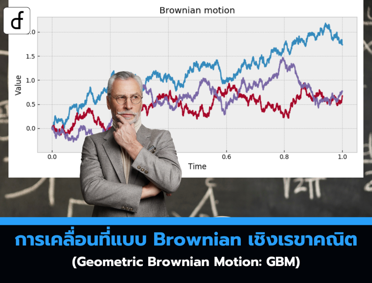
The usual model for the time-evolution of an asset price S(t) is given by the geometric Brownian motion, represented by the following stochastic differential equation:

$$\begin{array}{r}dS(t)=\mu S(t)dt+\sigma S(t)dB(t)\end{array}$$

Note that the coefficients $\mu$ and $\sigma$, representing the drift and volatility of the asset, respectively, are both constant in this model. In more sophisticated models they can be made to be functions of t, S(t) and other stochastic processes.

The solution S(t) can be found by the application of Ito's Lemma to the stochastic differential equation.

Dividing through by S(t) in the above equation leads to:

$$\begin{array}{r}\frac{dS(t)}{S(t)}=\mu dt+\sigma dB(t)\end{array}$$

Notice that the left hand side of this equation looks similar to the derivative of log S(t). Applying Ito's Lemma to log S(t) gives:

$$\begin{array}{r}d(logS(t))=(logS(t){)}^{\prime }\mu S(t)dt+(logS(t){)}^{\prime }\sigma S(t)dB(t)+\frac{1}{2}(logS(t){)}^{″}{\sigma }^{2}S(t{)}^{2}dt\end{array}$$

This becomes:

$$\begin{array}{r}d(logS(t))=\mu dt+\sigma dB(t)-\frac{1}{2}{\sigma }^{2}dt=(\mu -\frac{1}{2}{\sigma }^2)dt+\sigma dB(t)\end{array}$$

This is an Ito drift-diffusion process. It is a standard Brownian motion with a drift term. Since the above formula is simply shorthand for an integral formula, we can write this as:

$$\begin{array}{r}log(S(t))-log(S(0))=(\mu -\frac{1}{2}{\sigma }^2)t+\sigma B(t)\end{array}$$

Finally, taking the exponential of this equation gives:

$$\begin{array}{r}S(t)=S(0)\exp ((\mu -\frac{1}{2}{\sigma }^2)t+\sigma B(t))\end{array}$$

This is the solution the stochastic differential equation. In fact it is one of the only analytical solutions that can be obtained from stochastic differential equations.

Reference: Geometric Brownian Motion

From https://www.quantstart.com/articles/Geometric-Brownian-Motion/