Brownian Motion and Wiener Process

In a previous article on the website, we introduced stochastic calculus in the context of its role in quantitative finance. The properties of Markov and Martingale were also defined to prepare for the mathematical tools necessary for simulating asset price paths.

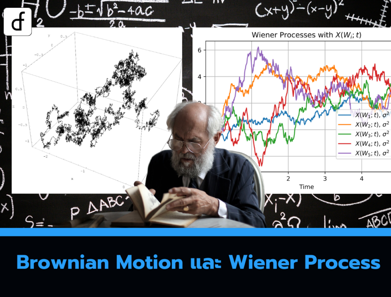
In both articles, it is stated that Brownian motion will be used as a model for the price paths of assets over time. In this article, Brownian motion will be formally defined and its mathematical derivative, the Wiener process, will be explained. It will be shown that standard Brownian motion is insufficient for modeling asset price movements, and geometric Brownian motion is more appropriate.

From the previous discussion on the properties of Markov and Martingale, there has been an experiment with discrete coin tossing using an arbitrary number of time intervals. The goal here is to move towards a continuous-time random walk, which will be a more complex model for asset prices that change over time. To achieve this goal, it is necessary to increase the number of time steps. However, the method of increasing must be done in a specific manner to avoid meaningless results (such as infinity).

Consider a continuous real-valued time interval $[0,T]$, with $T>0$. In this interval $N$ coin tosses will be carried out, which each take a time $T/N$. Hence the coin tosses will be spaced equally in time. Concurrently the payoff returned from each coin toss will be modified. The sequence of discrete random variables representing the coin toss is $Z_i\in \{-1,1\}$. A further sequence of discrete random variables, ${\tilde{Z}}_i\in \{\sqrt{T/N},-\sqrt{T/N}\}$, can also be defined. This definition of such a sequence of discrete random variables is used to provide a very specific quadratic variation of the coin toss.

The quadratic variation of a sequence DRVs are defined as the sum of the squared differences between the current value and the previous value:$$\begin{array}{r}\sum _{k=1}^i{(S_k-S_{k-1})}^2\end{array}$$

For $Z_i$, the first coin toss random variable sequence, the quadratic variation is given by:$$\begin{array}{r}\sum _{k=1}^i{(S_k-S_{k-1})}^2=i\end{array}$$

For ${\tilde{Z}}_i$ the quadratic variation of the partial sums ${\tilde{S}}_i$ is:

$$\begin{array}{r}\sum _{k=1}^N{({\tilde{S}}_k-{\tilde{S}}_{k-1})}^2=N\times {\left(\sqrt{\frac{T}{N}}\right)}^2=T\end{array}$$

Thus, by construction, the quadratic variation of the amended coin toss ${\tilde{Z}}_i$ is simply the total duration of all tosses, $T$.

Importantly, note that both the Markov and Martingale properties are retained by ${\tilde{Z}}_i$. As $N\to \mathrm{\infty }$ the random walk coin toss does not diverge. If the value of the asset at time $t$, with $t\in [0,T]$, is given by $S(t)$, then its conditional expectation at the end of the interval, given that $S(0)=0$, is $\mathbb{E}(S(T))=0$ with a variance of $\mathbb{E}(S(T{)}^2)=T$.

Even though the technical details are not mentioned, when the number of steps N approaches infinity, we obtain the Wiener process, commonly referred to as standard Brownian motion, denoted by B(t), with the formal definition as follows:

The sequence of random variables B(t) is Brownian motion. If B(0) = 0 and for all t, s where s < t, B(t) - B(s) is normally distributed with variance t - s, and the distribution of B(t) - B(s) is independent of B(r) for 

Properties of Brownian Motion

• Brownian motions are finite: The construction  is carefully designed so that when N is large, B remains finite and non-zero.
• Brownian motions have unbounded variation: This means that if all the negative slope signals are switched to positive, B can increase to infinity within a short period.
• Brownian motions are continuous: Although they are continuous at every point, derivatives cannot be found anywhere. This means that Brownian motion has fractal geometry, which significantly affects the choice of calculus methods used when analyzing or managing Brownian motion.
• Brownian motions are consistent with both the properties of Markov and Martingale: The conditional distribution of B(t) given information up to s depends only on t - s, and given information up to s, the conditional expectation of B(t) is B(s).
• Brownian motions are strongly normally distributed: This means that for t > s, the value of B(t) - B(s) is normally distributed with a mean of zero and a variance of t - s.